Introduction
So you obtained a nifty neurotechnology gadget? And now you would like to work with the data in your favorite development environment? In the past it took me months to achieve this, but thanks to BrainFlow it can work in minutes! Let me show you how I did it.
Most of the code should work for any device, but I will use the OYMotion gForcePro armband we used in a past project. It streams 8 channels of electromyographic (EMG) data at 500 Hz. I just want to see this data realtime in a plot. In the past I always used Python for this task, but the experience was not smooth, because it had difficulties with handling this high data rate. I could try to write everything in c++, but that would take me ages. I recently found the Julia language, which is aimed to be both fast and easy to use. With Julia I succeeded with ease, so I’ll show you how to visualize the data in Julia.
Installing BrainFlow.jl
Assuming you have Julia installed, you should start by adding the BrainFlow.jl package. Since BrainFlow 3.8.1 we have an automated Julia package, which installs everything for you. Adding packages in Julia is easy with the internal Julia package manager, just type in the Julia REPL:
using Pkg
Pkg.add("BrainFlow")
This may take a moment, since it has to download the compiled BrainFlow C++ libraries.
Starting small
Let’s start by acquiring a small data sample and plotting it. We’ll get to streaming the data later.
First we have to connect to the gForcePro device using BrainFlow. You can find how to do this in other languages in the BrainFlow docs examples section.
using BrainFlow
BrainFlow.enable_dev_logger(BrainFlow.BOARD_CONTROLLER)
params = BrainFlowInputParams()
board_shim = BrainFlow.BoardShim(BrainFlow.GFORCE_PRO_BOARD, params)
BrainFlow.prepare_session(board_shim)
BrainFlow.start_stream(board_shim)
You should receive some messages that you are succesfull, such as:
[2021-01-04 20:00:52.424] [brainflow_logger] [debug] start streaming
That’s it! I assume the code is pretty self-explanatory.
Once the stream is started, you can make some gestures. Then you get the collected data from BrainFlow directly via:
data = BrainFlow.get_board_data(board_shim) |> transpose
The output data is a matrix where the columns are the available channels and the rows are the samples. Andrey from BrainFlow tranposed the matrix, because he didn’t yet know Julia is column-major, so I transposed it back. We may remove this transpose in a future version, so beware.
This data matrix has 10 channels, while we know the gForce armband has only 8 EMG channels. We can easily get the EMG channels as follows:
emg_channels = BrainFlow.get_emg_channels(BrainFlow.GFORCE_PRO_BOARD)
emg_data = data[:, emg_channels]
It turns out channel 2:9 are for EMG data. The first column is actually a package identifier related to how the gForce sends the data, the 10th column is a timestamp we could also use if we want. The function BrainFlow.get_timestamp_channel could have told us that. An overview of which channels are available in which board would be a nice addition to the BrainFlow documentation. Feel free to become an open source contributor ;)
Now let’s make a plot from the data. For this single static plot, I’ll use the VegaLite.jl package. The plotting eco-system around Julia is still evolving rapidly with Plots.jl, Makie.jl and more, but I like these grammar of graphics style interfaces like ggplot from R. VegaLite provides such a grammar of graphics and VegaLite.jl is a Julia wrapper around it.
In order to best use VegaLite, we first create a dataframe using DataFrames.jl.
df = DataFrame(emg_data)
emg_names = Symbol.(["emg$x" for x in 1:8])
DataFrames.rename!(df, emg_names)
Let’s also add a time column for use as x-axis. I could probably use the timestamp channel, but I’m lazy and will just construct it on the fly from the number of rows:
sampling_rate = BrainFlow.get_sampling_rate(BrainFlow.GFORCE_PRO_BOARD)
nrows = size(df)[1]
df.time = (1:nrows)/sampling_rate
Now you should have a dataframe with some named EMG columns and a time column:
julia> df
2576×9 DataFrame
  Row │ emg1     emg2     emg3     emg4     emg5     emg6     emg7     emg8     time
      │ Float64  Float64  Float64  Float64  Float64  Float64  Float64  Float64  Float64
──────┼─────────────────────────────────────────────────────────────────────────────────
    1 │ 31095.0  31342.0  29554.0  30069.0  31095.0  31860.0  29299.0  30069.0    0.002
  ⋮   │    ⋮        ⋮        ⋮        ⋮        ⋮        ⋮        ⋮        ⋮        ⋮
2575 rows omitted
The Grammar of Graphics is a little special, it’s typically best to go for the most tall dataframe as possible. You’ll see in a moment why, but let’s just stack all the emg channels into two columns:
df2 = stack(df, 1:8)
rename!(df2, [:time, :channel, :value])
Now we have a dataframe with the channel values stacked in one column, and the channel names in another column:
julia> df2
20608×3 DataFrame
   Row │ time     channel  value
       │ Float64  String   Float64
───────┼───────────────────────────
     1 │   0.002  emg1     31095.0
   ⋮   │    ⋮        ⋮        ⋮
20607 rows omitted
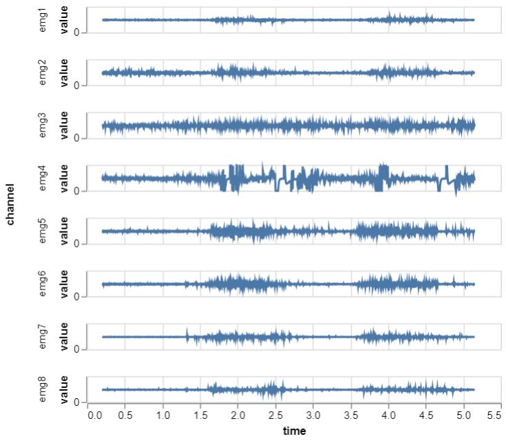
Alright, that’s it. Now we can start plotting. Well… one last thing I quickly filtered the start of the signals with Query.jl, because the data was a bit spikey there due to somekind of startup effect. Ok for real now, let’s pipe it into a VegaLite plot:
df2 |> @filter(_.time > 0.2) |>
@vlplot(
    :line,
    x=:time,
    y=:value,
    row=:channel,
    width=400,
    height=25
)
What I love about this grammar of graphics is that you can quickly configure your plot based on your columns. Here I choose the time column as x-axis, the values as y-axis and the named EMG channels as rows resulting in the following plot:
Done! If you want the whole thing, I placed the full script here. There’s plenty of additional playing and tinkering we could do with this, but I want to move on to the real stuff.
Streaming data visualization
Because we want to visualize the live data. You can see the final result below, where we make a few gestures and watch the biosignals unfold right in front of your eyes. It’s always a magical moment!
So how did I succeed in doing this? It was a bit more work than making a single VegaLite plot, so I placed the code in thisBrainFlowViz.jl repository. The gForce visualization script is in /test/brainflow_gforce.jl. Let’s walk you through it.
Parsing the data
First make sure the BrainFlow has started a stream, just like in the previous section.
Then I wrote a custom function to acquire some EMG data and detrend it.
function get_some_board_data(board_shim, nsamples)
    data = BrainFlow.get_current_board_data(nsamples, board_shim)
    data = transpose(data)
    emg_data = view(data, :, 2:9)
    for chan in 1:8
        emg_channel_data = view(emg_data, :, chan)
        BrainFlow.detrend(emg_channel_data, BrainFlow.CONSTANT)
    end
    return emg_data
end
The function BrainFlow.get_current_board_data is slightly different from BrainFlow.get_board_data in that it retrieves only the last n-samples of data and does not clear the internal BrainFlow buffer. This will be helpful for continuously requesting a slice of data and plotting it. Beware that at the very start of the stream the internal buffer is not yet full, so you may get a matrix with less rows than the requested number of samples.
Next I select the EMG data channels as a view for performance, because that creates a kind of reference to the data instead of making a copy.
In a quick for-loop, I then continue to detrend each ‘viewed’ EMG channel individual with BrainFlow.detrend(). A constant detrend means we just remove the average per channel. I could probably have done this efficiently with some Julia code, but wanted to try out calling a BrainFlow data filtering function from Julia. This function directly passes an array from Julia to the BrainFlow c++ libraries, using the same allocated memory.
As a small interlude, you can read the BrainFlow julia-package source code you would see just how easy it is to do this in Julia:
ccall((:detrend, DATA_HANDLER_INTERFACE), Cint, (Ptr{Float64}, Cint, Cint), data, length(data), Int32(operation))
One line of code! I won’t go into the details, but I dare you to do these tricks yourself in Cython or Rcpp or MATLAB’s MEX framework. This is one of the reason I love Julia, integration with c/c++ is pretty much seamless.
We are now ready to start plotting the data.
Plotting the data
I made a nice convenience function for plotting the BrainFlow data from any data retrieval function. Here’s what I used to make my video. Beforehand, I called the get_some_board_data() function once while wearing the armband to check what would be good y-scale limits.
using BrainFlowViz
nchannels = 8
nsamples = 512
data_func = ()->get_some_board_data(board_shim, nsamples)

BrainFlowViz.plot_data(
    data_func,
    nsamples,
    nchannels;
    y_lim = [-1300 1300],
    theme = :dark,
    color = :lime,
    )
Alright, but how does this work internally? To plot the animated data I did not use VegaLite.jl because it is not suitable for high performance animations. For that reason I choose Makie.jl which calls itself a high-performance, extendable, and multi-platform plotting ecosystem for the Julia programming language. It also has an optional WebGL backend in case I want to move to a web-based application.
I used the Makie documentation to find my way. First I needed an array of Nodes, or actuallyObservables, which I fill with the EMG data. Whenever a Node changes, Makie will refresh the plot for you. That’s very convenient! Just to be sure we are performant I push views of the EMG data into each Node. Remember, we don’t like copying data for no reason!
xs = collect(1:nsamples) # data for the x-axis
ys = [] # array of data per channel for the y-axis
for n = 1:nchannels
    push!(ys, Node(view(emg_data, :, n)))
end
To start with Makie and multiple plots, you need a Scene with a layout. This interface is available in the AbstractPlotting package, so we also need that package. We then populate this layout with a bunch of axes with lines in it.
Note: your first initial plot may take a while in Julia. Julia compiles the source code ahead-of-time upon the first function call (unless you explicitly compiled it yourself beforehand with PackageCompiler.jl). That means the first function call is slower than all the other subsequent calls. That’s fine for an animation with lots of frames like we need. Just don’t be too alarmed about things taking a moment. And the Julia development community is rapidly speeding up the compilation, so this will get better and better.
Now let’s make that initial scene:
using Makie, AbstractPlotting

outer_padding = 30
scene, layout = layoutscene(
    outer_padding,
    resolution = (1200, 700),
    backgroundcolor = RGBf0(0.99, 0.99, 0.99),
)

ax = Array{LAxis, 1}(undef, nchannels)
for n = 1:nchannels
    ax[n] = layout[n, 1] = LAxis(scene, ylabel = "ch$n")
    lines!(ax[n], xs, ys[n], color = color, linewidth = 2)
end
Now while the EMG data is streaming we need to acquire it and update the y-axis Nodes. Remember that Makie will refresh the plot for us if we do that right. So you need something like this:
while(true)
    sleep(delay) # wait a small moment (use a time interval below your desired frame rate)

    # get some new data, remember this calls get_some_board_data()
    emg_data = data_func()

    # update each Node individually
    for n = 1:nchannels
        ys[n][] = view(emg_data, :, n)
    end
end
Well that was it. Yes, really! Ofcourse you can further tinker with it. For example, change all the axes properties to get a dark theme like I created, but that’s just details you can find in the Makie documentation.
Parallel processing
Ok, one last thing.
This animated plot will block your REPL, because it uses the same thread. You can kill it with ctrl+c, but if you want some easy parallel processing you can use Julia tasks. Again this is trivial, just create a task using the macro and schedule it:
t = @task BrainFlowViz.plot_data(...)
sleep(0.5) # sometimes I have to give it a little time
schedule(t)
You can stop the task by scheduling an InterruptException, which is similar to what happens when you hit ctrl+c:
schedule(t, InterruptException(), error=true)
Conclusion
I showed you how I visualized the streaming data from the gForcePro armband. For me it was a very smooth experience and I hope you learned just how easy it is nowadays to get started with your bio-sensor data. Please reach out if you do things with BrainFlow! You can also join our BrainFlow Slack channel if you have further questions or suggestions.